6 Differential Abundance Analysis
6.1 Using difftest from microbial package
The difftest() function from the microbial package serves as a robust solution for conducting differential abundance testing in microbiome data analysis. Its core objective is to identify taxa (such as bacteria and fungi) that demonstrate noteworthy differences in abundance levels across two or more groups of samples.
# Load required packages
library(microbial)

# Perform differential abundance analysis using difftest function
result_difftest <- difftest(ps_raw, group = "nationality")

# View the results
head(result_difftest[, 1:7])
         baseMean log2FoldChange     lfcSE      stat       pvalue         padj
OTU016 273.896003    -0.45871007 0.1610307 -2.848589 4.391364e-03 8.499414e-03
OTU038  18.625971     0.08889349 0.1401160  0.634428 5.258016e-01 6.504762e-01
OTU055  26.476581     0.44866807 0.1357274  3.305657 9.475402e-04 2.105645e-03
OTU095   8.707940    -1.44945993 0.1622408 -8.934006 4.108545e-19 3.081409e-18
OTU044   7.779078    -1.46593273 0.1931797 -7.588441 3.237768e-14 1.766055e-13
OTU097   1.633998     0.38558799 0.1657909  2.325749 2.003192e-02 3.338653e-02
       Sample-1
OTU016       87
OTU038       10
OTU055       15
OTU095        3
OTU044        8
OTU097        1
library(tidyverse)
library(ggtext)
library(microbial)
library(kableExtra)


result_difftest %>%
  select(log2FoldChange, pvalue, padj, Significant) %>%
  filter(Significant == "check") %>%
  filter(padj <= 0.05) %>%
  head(10) %>%
  kbl(caption = "Differential abundance results") %>%
kable_styling(bootstrap_options = "basic", full_width = F, position = "float_left")| log2FoldChange | pvalue | padj | Significant |
|---|---|---|---|
### Differential abundance plot

library(dplyr)
library(microbial)

difftest_w_metadata <- result_difftest %>%
  rename_all(~ make.unique(tolower(.), sep = "_")) %>%
  tibble::rownames_to_column("otu") %>%
  inner_join(., psmelt(ps_raw), by = c("otu" = "OTU")) %>%
  relocate(c(nationality, bmi_group), .after = otu) %>%
  mutate(nationality = factor(nationality,
                      levels = c("AAM", "AFR"),
                      labels = c("African American", "African")),
         bmi_group = factor(bmi_group,
                      levels = c("lean", "overweight", "obese"),
                      labels = c("Lean", "Overweight", "Obese"))) %>%
  rename_all(~ make.unique(tolower(.), sep = "_")) %>%
  select(-phylum_1, -family_1, -genus_1) %>%
  distinct(otu, .keep_all = TRUE) %>%
  pivot_longer(cols = c("phylum", "family", "genus"), names_to = "level", values_to = "taxon") %>%
  mutate(taxon = str_replace(string = taxon,
                            pattern = "(.*)",
                            replacement = "*\\1*"),
        taxon = str_replace(string = taxon,
                            pattern = "\\*(.*)_unclassified\\*",
                            replacement = "Unclassified<br>*\\1*"),
        taxon = str_replace_all(taxon, "_", " ")) %>%
  filter(padj <= 0.0001) %>%
  filter(level == "genus")

difftest_w_metadata %>%
  ggplot(aes(y = reorder(taxon, log2foldchange), x = log2foldchange, fill = nationality)) +
  geom_col() +
  theme_light() +
  labs(x = "Log2 Fold Change", y = "", fill = NULL, subtitle = "Differential abundance by nationality") +
  theme(axis.text.y = element_markdown(size = 7),
        legend.text = element_markdown(size = 7)) +
  coord_cartesian(xlim = c(-3, 4))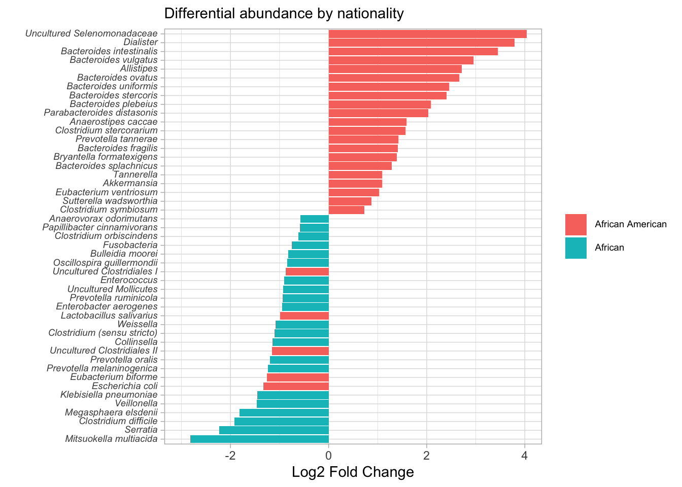
difftest_w_metadata %>%
  ggplot(aes(y = reorder(taxon, log2foldchange), x = log2foldchange, fill = bmi_group)) +
  geom_col() +
  theme_light() +
  labs(x = "Log2 Fold Change", y = "", fill = NULL, subtitle = "Differential abundance by BMI") +
  theme(axis.text.y = element_markdown(size = 7),
        legend.text = element_markdown(size = 7)) +
  coord_cartesian(xlim = c(-3, 4))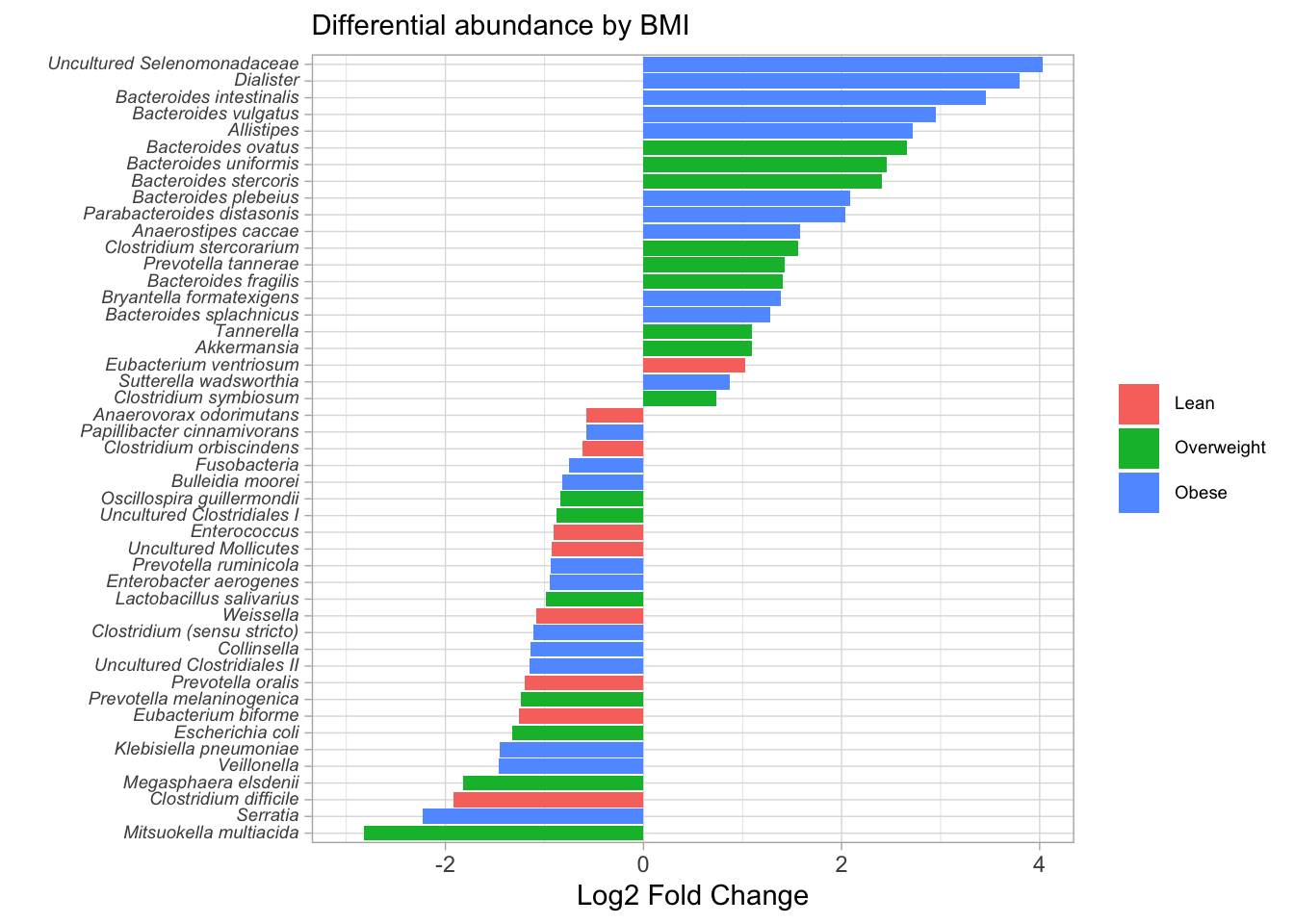
save(difftest_w_metadata, file = "data/difftest_w_metadata.rda")Practicing with filtering and pivot_longer()
library(purrr)
library(dplyr)
library(tidyr)
sig_genera <- difftest_w_metadata %>%
arrange(padj) %>%
select(taxon, nationality, bmi_group, basemean, log2foldchange, lfcse, stat, pvalue, padj, "sample-1":"sample-222") %>%
pivot_longer(cols = c("sample-1":"sample-222"), names_to = "sample_id", values_to = "count") %>%
group_by(sample_id) %>%
mutate(rel_abund = count/sum(count)) %>%
ungroup() %>%
dplyr::select(-count) %>%
relocate(sample_id) %>%
filter(rel_abund > 0.1) %>%
filter(padj < 0.01)
head(sig_genera)
# A tibble: 6 × 11
sample_id taxon nationality bmi_group basemean log2foldchange lfcse stat
<chr> <chr> <fct> <fct> <dbl> <dbl> <dbl> <dbl>
1 sample-128 *Bactero… African Am… Overweig… 106. 2.66 0.148 18.0
2 sample-39 *Allisti… African Am… Obese 246. 2.72 0.158 17.2
3 sample-45 *Allisti… African Am… Obese 246. 2.72 0.158 17.2
4 sample-68 *Allisti… African Am… Obese 246. 2.72 0.158 17.2
5 sample-73 *Allisti… African Am… Obese 246. 2.72 0.158 17.2
6 sample-109 *Allisti… African Am… Obese 246. 2.72 0.158 17.2
# ℹ 3 more variables: pvalue <dbl>, padj <dbl>, rel_abund <dbl>
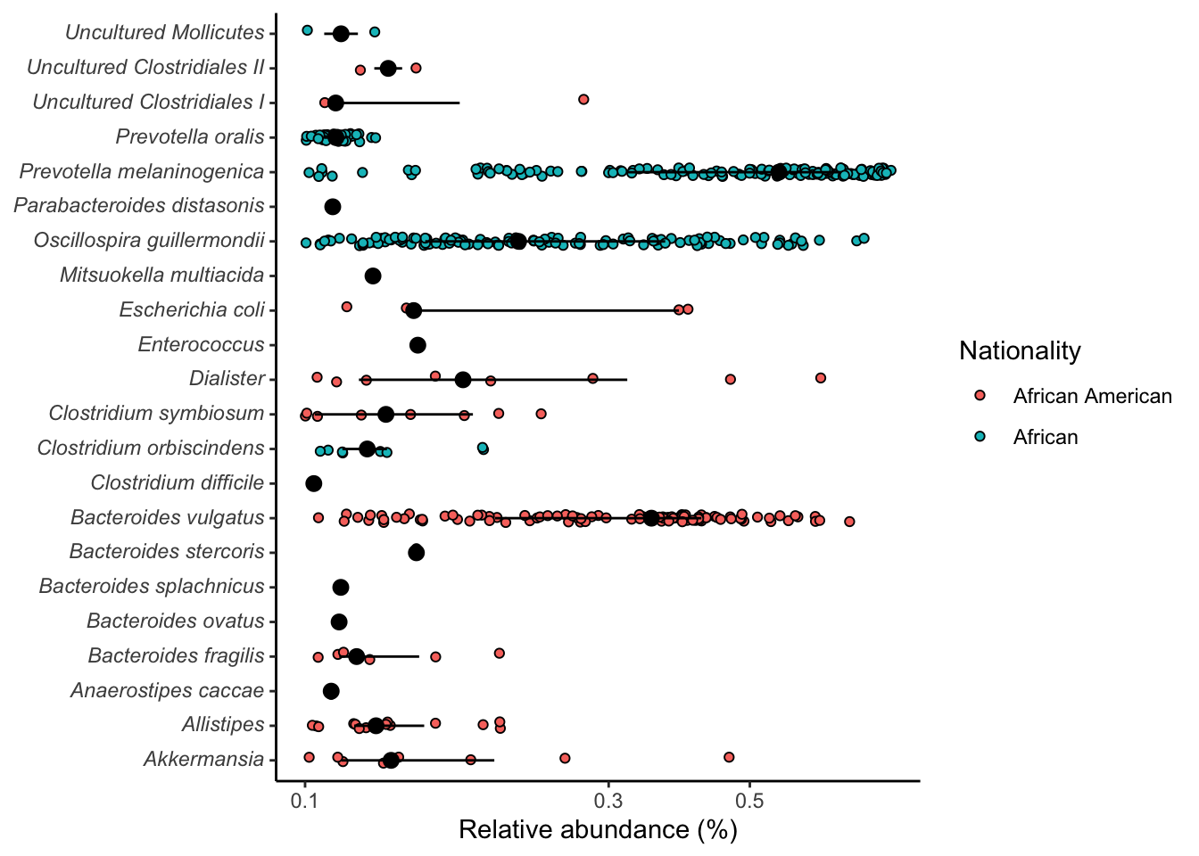
# By nationality
sig_genera %>%
ggplot(aes(x=rel_abund, y=taxon, fill = nationality)) +
geom_jitter(position = position_jitterdodge(dodge.width = 0.8,
jitter.width = 0.5),
shape=21) +
stat_summary(fun.data = median_hilow, fun.args = list(conf.int=0.5),
geom="pointrange",
position = position_dodge(width=0.8),
show.legend = FALSE) +
scale_x_log10() +
scale_color_manual(NULL,
breaks = c(F, T),
values = c("grey", "dodgerblue"),
labels = c("African American", "African")) +
labs(x= "Relative abundance (%)", y=NULL, fill = "Nationality") +
theme_classic() +
theme(
axis.text.y = element_markdown()
)
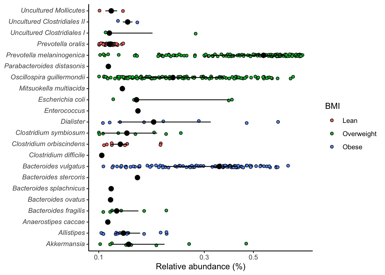
# By body mass index
sig_genera %>%
  ggplot(aes(x=rel_abund, y=taxon, fill = bmi_group)) +
  geom_jitter(position = position_jitterdodge(dodge.width = 0.8,
                                              jitter.width = 0.5),
              shape=21) +
  stat_summary(fun.data = median_hilow, fun.args = list(conf.int=0.5),
               geom="pointrange",
               position = position_dodge(width=0.8),
               show.legend = FALSE) +
  scale_x_log10() +
  labs(x= "Relative abundance (%)", y=NULL, fill = "BMI") +
  theme_classic() +
  theme(
    axis.text.y = element_markdown()
)
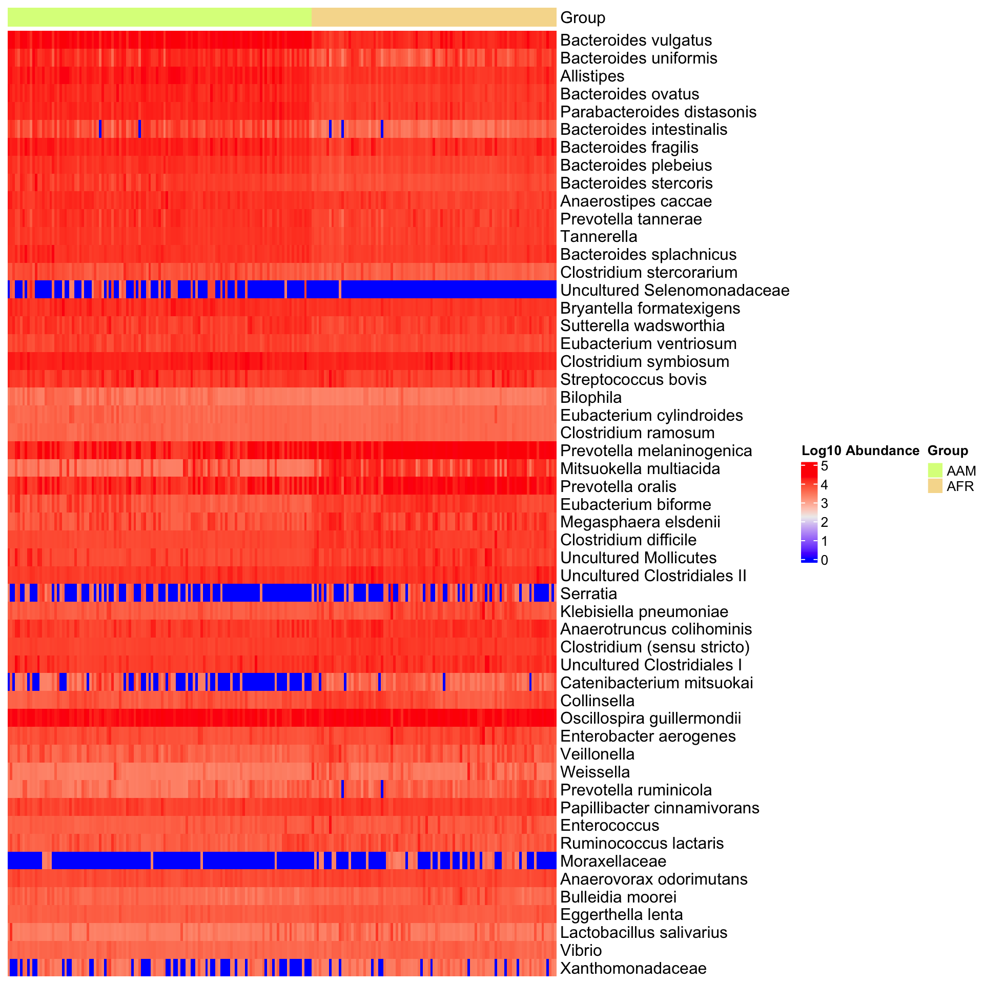
ggsave("figures/significant_genera.tiff", width=6, height=4)6.2 Using run_lefse() in microbiomeMaker Package
The run_lefse() function in the microbiomeMaker R package provides a convenient method for performing Differential Abundance Analysis on microbiome data. By leveraging the Linear Discriminant Analysis Effect Size (LEfSe) algorithm, run_lefse() enables researchers to interpret the results in the context of biological class labels, uncovering important insights into microbial community dynamics.
library(phyloseq)
library(microbiomeMarker)

# Run LEfSe analysis
run_lefse(
  ps_raw,
  wilcoxon_cutoff = 0.0001,
  group = "nationality",
  taxa_rank = "Genus",
  transform = "log10p",
  kw_cutoff = 0.01,
  multigrp_strat = TRUE,
  lda_cutoff = 2
) %>%
plot_heatmap(group = "nationality", color = "rainbow")