5 Differential Analysis of Microbiome Data

Differential abundance analysis is a fundamental technique in microbiome research used to identify features that exhibit significant differences in abundance across different biological conditions or treatments. This analysis is crucial for understanding the dynamics of microbial communities and their response to various environmental factors. In this section, we will explore different methods for conducting differential abundance analysis using microbiome data.

5.1 Using run_lefse() in microbiomeMaker Package

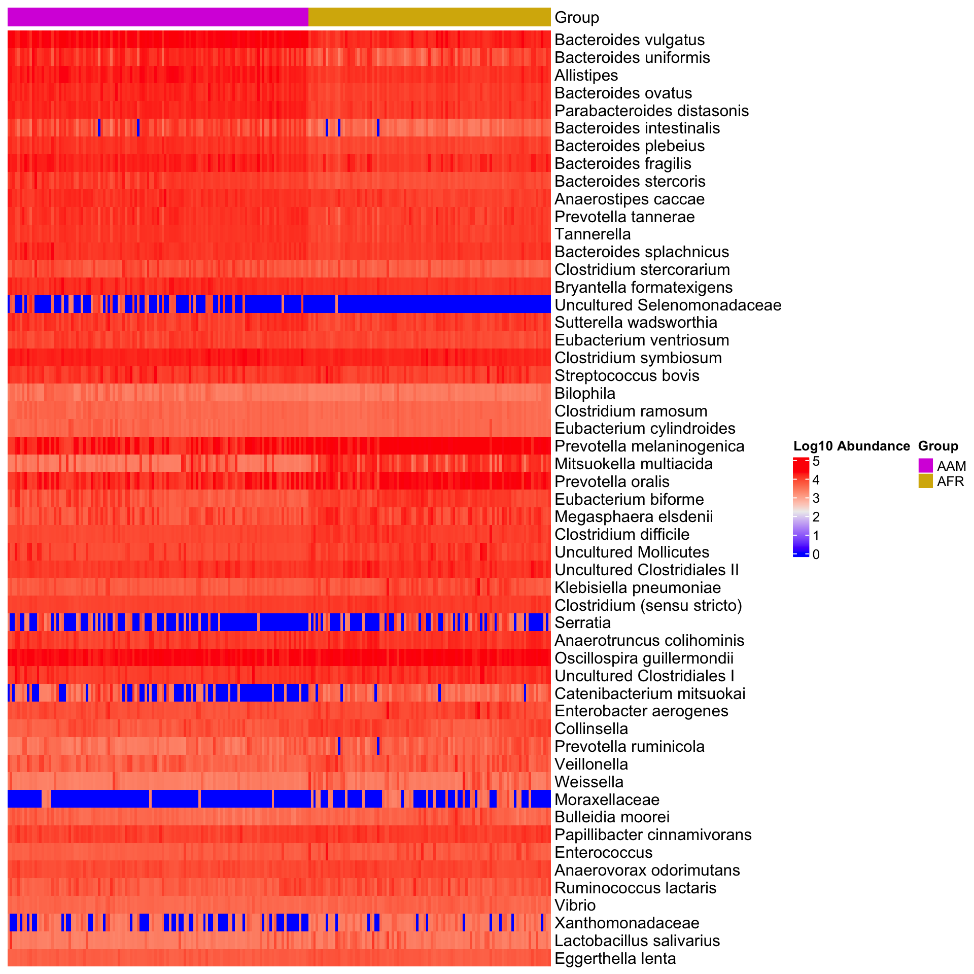
The run_lefse() function in the microbiomeMaker R package provides a convenient method for performing Differential Abundance Analysis on microbiome data. By leveraging the Linear Discriminant Analysis Effect Size (LEfSe) algorithm, run_lefse() enables researchers to interpret the results in the context of biological class labels, uncovering important insights into microbial community dynamics.

Dataset: dietswap

library(phyloseq)
library(microbiomeMarker)

# Run LEfSe analysis
run_lefse(
  psextra_raw,
  wilcoxon_cutoff = 0.0001,
  group = "nationality",
  taxa_rank = "Genus",
  transform = "log10p",
  kw_cutoff = 0.01,
  multigrp_strat = TRUE,
  lda_cutoff = 2
) %>% 
plot_heatmap(group = "nationality", color = "rainbow")

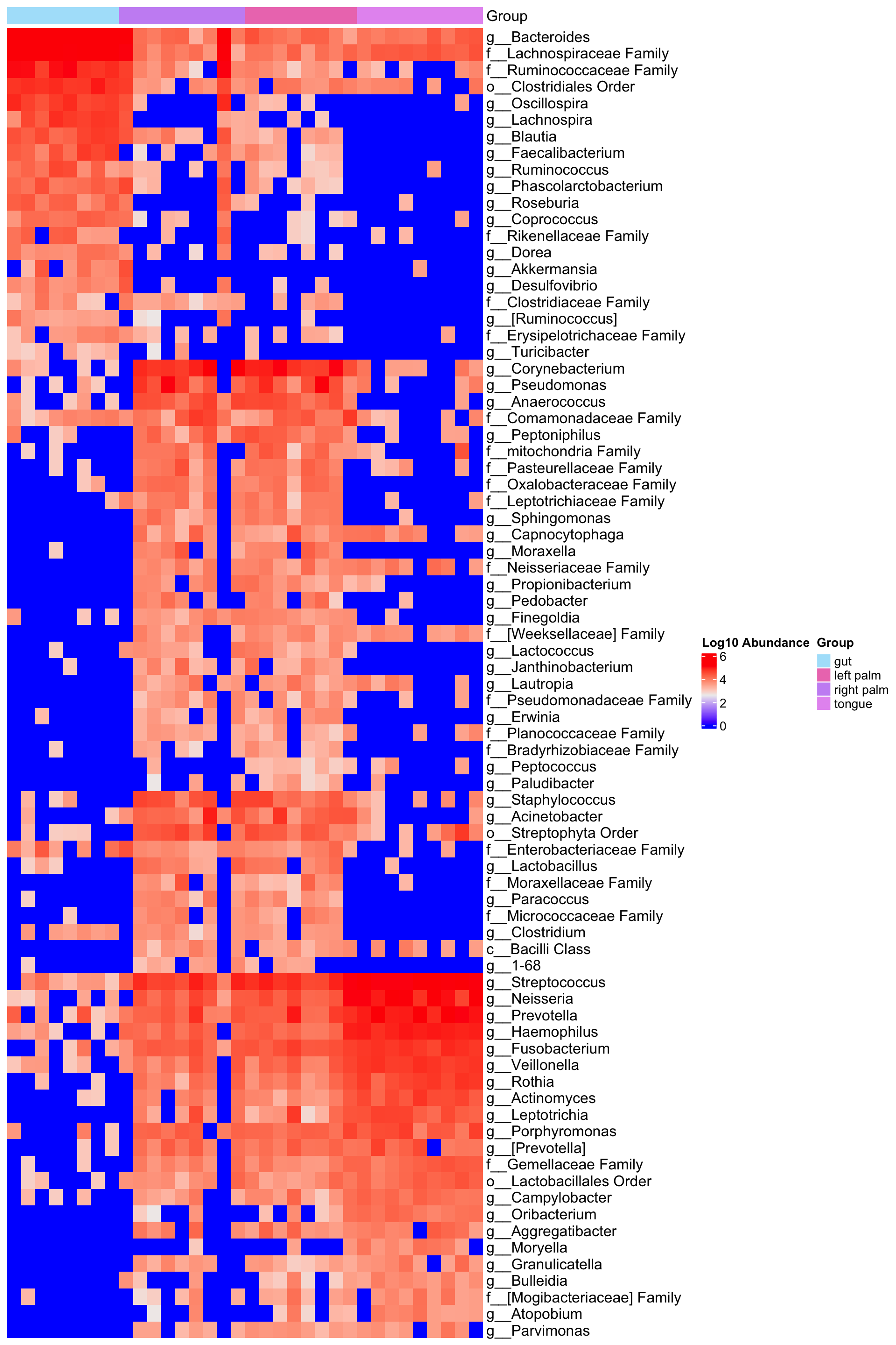
Dataset: caporaso

library(microbiomeMarker)

ps_caporaso <- ps_caporaso %>%  tax_fix()

run_lefse(
    ps_caporaso, 
    wilcoxon_cutoff = 0.001,
    group = "SampleType",
    taxa_rank = "Genus",
    transform = "log10p",
    kw_cutoff = 0.01,
    multigrp_strat = TRUE,
    lda_cutoff = 2) %>%
  plot_heatmap(group = "SampleType", color = "rainbow")

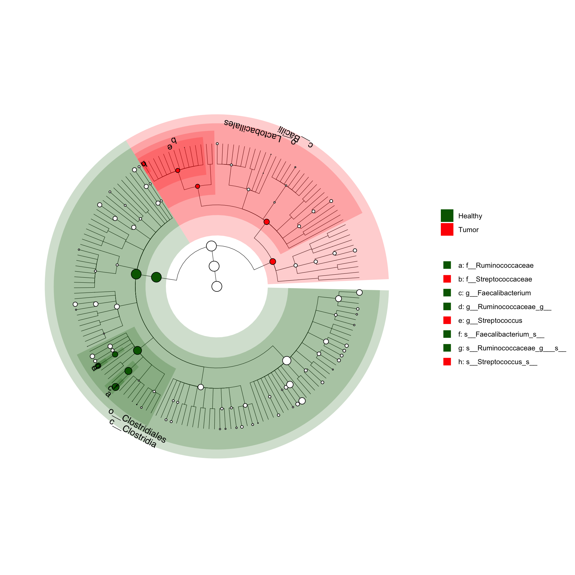
5.2 Cladogram on kostic_crc dataset

Using plot_cladogram() from microbiomeMarker package

library(microbiomeMarker)
kostic_crc_small <- phyloseq::subset_taxa(
    ps_kostic_crc,
    Phylum %in% c("Firmicutes")
)
mm_lefse <- run_lefse(
    kostic_crc_small,
    wilcoxon_cutoff = 0.01,
    group = "DIAGNOSIS",
    kw_cutoff = 0.01,
    multigrp_strat = TRUE,
    lda_cutoff = 4
)
plot_cladogram(mm_lefse, color = c("darkgreen", "red"))