7 Patterns and Associations Analysis
In this section, we will explore methods for analyzing patterns and associations within datasets. These methods are instrumental in uncovering relationships between variables, identifying underlying patterns, and elucidating complex structures within the data. Specifically, we will discuss correlation analysis, heatmap visualization, hierarchical clustering, and other techniques for exploring patterns and associations in various types of datasets.
7.1 Correlation analysis and visualization
Correlation analysis quantifies the strength and direction of the linear relationship between two continuous variables. It helps in understanding how variables are related to each other and can identify potential associations or dependencies within the data. Heatmap visualization is commonly integrated with correlation analysis to visually represent correlation matrices, allowing for the identification of patterns and relationships between variables.
7.1.1 Pearson Correlation Heatmap with microViz Package
In this section, we utilize the cor_heatmap function available in the microViz package to generate a heatmap visualizing Pearson correlation coefficients between variables. This technique allows for the exploration of relationships and patterns within the data, providing insights into the strength and direction of linear associations between variables.
ps_extra <- ps_dietswap %>%
tax_transform(
  trans = "clr",
  rank = "Genus",
  keep_counts = TRUE,
  zero_replace = 0,
  add = 0,
  transformation = NULL
)
# Load required packages
library(phyloseq)
library(microViz)

# Set up the data with numerical variables and filter to top taxa
ps <- ps_dietswap %>%
  ps_mutate(
    bmi = recode(bmi_group, obese = 3, overweight = 2, lean = 1),
    female = if_else(sex == "female", true = 1, false = 0),
    african = if_else(nationality == "AFR", true = 1, false = 0)
  ) %>%
  tax_filter(
    tax_level = "Genus", min_prevalence = 1 / 10, min_sample_abundance = 1 / 10
  ) %>%
  tax_transform("identity", rank = "Genus")

# Randomly select 30 taxa from the 50 most abundant taxa (just for demo)
set.seed(123)
top_taxa <- tax_top(ps_dietswap, n = 10, by = sum, rank = "unique", use_counts = FALSE)

taxa <- sample(tax_top(ps_dietswap, n = 50), size = 30)

# Clean the data and draw the correlation heatmap
cor_heatmap(
  data = ps,
  taxa = taxa,
  taxon_renamer = function(x) stringr::str_remove(x, " [ae]t rel."),
  tax_anno = taxAnnotation(
    Prev. = anno_tax_prev(undetected = 50),
    Log2 = anno_tax_box(undetected = 50, trans = "log2", zero_replace = 1)
  )
)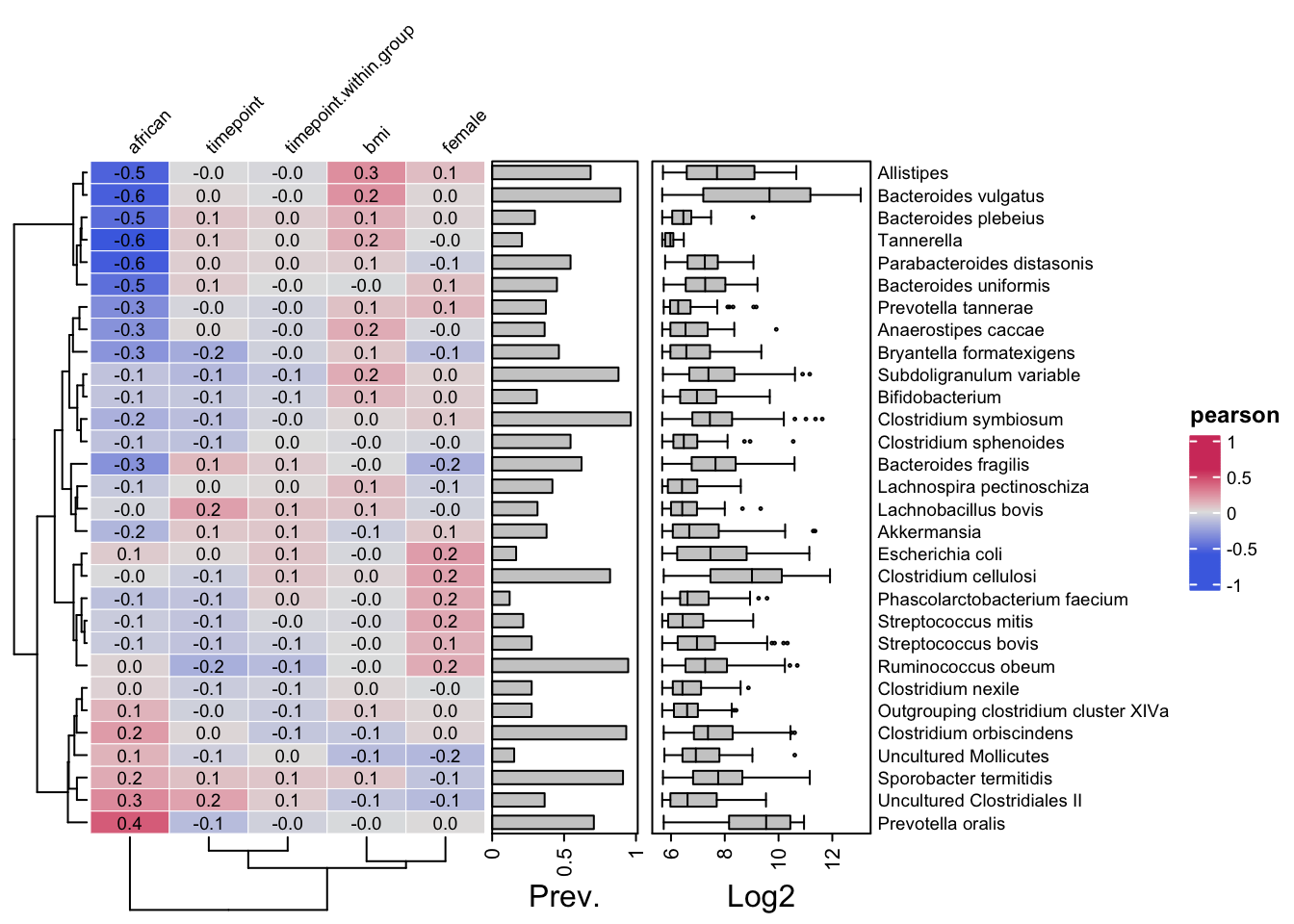
Note: The parameter min_prevalence = 0.1 is set, equivalent to approximately 23 out of 222 samples. This value may vary depending on the dataset. Adjust as necessary.
7.2 Hierarchical clustering
Hierarchical clustering is a method for grouping similar observations or variables together based on their similarity or dissimilarity. It creates a hierarchical tree-like structure (dendrogram) that illustrates the relationships between clusters, allowing for the identification of natural groupings or patterns within the data.