6 Data Splitting

The dataset is divided into separate subsets for training and testing. This partitioning allows for an unbiased evaluation of the model’s performance on unseen data, helping to assess its ability to generalize to new observations.

6.1 Load necessary libraries

set.seed(1234)



# Load necessary libraries
library(caret)
library(tidyverse)

# Example dataset (replace with your own data)

load("data/data_imputed.rda")
data <- data_imputed #%>%
  # mutate(target_text = dplyr::recode_factor(target, "0" = "AAM", "1" = "AFR"), .after = 1)

6.2 Split using caret::createDataPartition()

# Split data into training and testing sets
set.seed(123) # for reproducibility
train_index <- caret::createDataPartition(data$target, p = 0.8, list = FALSE)
train_data <- data[train_index, ]
test_data <- data[-train_index, ]

write_csv(test_data, "models/test_data.csv")

save(train_data, test_data, file = "data/train_test_data.rda")

6.3 Review train and test datasets

cat("\nDimension of the train data using caret package\n is", base::dim(train_data)[1], "rows and", base::dim(train_data)[2], "columns.\n")

Dimension of the train data using caret package
 is 179 rows and 144 columns.
cat("\nDimension of the test data using caret package\n is", base::dim(test_data)[1], "rows and", base::dim(test_data)[2], "columns.\n")

Dimension of the test data using caret package
 is 43 rows and 144 columns.

cat("\nThe intersection between test and train dataset is", nrow(test_data %>% intersect(train_data)))

The intersection between test and train dataset is 0

6.4 Spliting using dplyr::sample_n() and dplyr::setdiff() functions**

set.seed(123)

library(dplyr)
test_df = train_data %>% dplyr::sample_n(0.2*nrow(train_data))
train_df = train_data %>% dplyr::setdiff(test_df)

cat("\nDimension of the test data using dplyr package\n is", base::dim(test_df)[1], "rows and", base::dim(test_df)[2], "columns.\n")

Dimension of the test data using dplyr package
 is 35 rows and 144 columns.
cat("\nDimension of the train data using dplyr package\n is", base::dim(train_df)[1], "rows and", base::dim(train_df)[2], "columns.\n")

Dimension of the train data using dplyr package
 is 144 rows and 144 columns.

cat("\nThe intersection between test and train dataset is", nrow(test_df %>% intersect(train_df)))

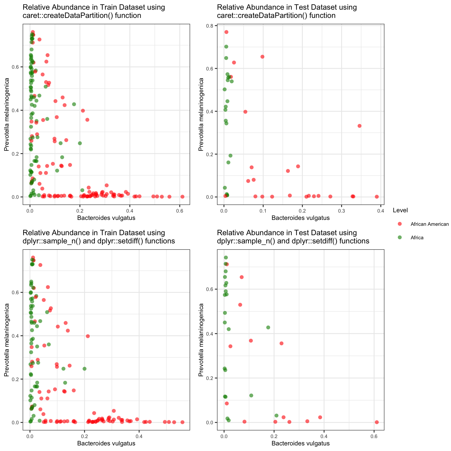
The intersection between test and train dataset is 0

6.5 Relative abundance in training and testing datasets

library(dplyr)
library(ggplot2)
library(ggpubr)

cols <- c("0" = "red","1" = "green4")

p1 <- train_data %>% ggplot(aes(x = `Bacteroides vulgatus`, y = `Prevotella melaninogenica`, color = factor(target))) + geom_point(size = 2, shape = 16, alpha = 0.6) +
  labs(title = "Relative Abundance in Train Dataset using \ncaret::createDataPartition() function") +
  scale_colour_manual(values = cols, labels = c("African American", "Africa"), name="Level") +
  theme_bw() +
  theme(text = element_text(size = 8))

p2 <- test_data %>% ggplot(aes(x = `Bacteroides vulgatus`, y = `Prevotella melaninogenica`, color = factor(target))) + geom_point(size = 2, shape = 16, alpha = 0.6) +
  labs(title = "Relative Abundance in Test Dataset using \ncaret::createDataPartition() function") +
  scale_colour_manual(values = cols, labels = c("African American", "Africa"), name="Level") +
  theme_bw() +
  theme(text = element_text(size = 8))


p3 <- train_df %>% ggplot(aes(x = `Bacteroides vulgatus`, y = `Prevotella melaninogenica`, color = factor(target))) + geom_point(size = 2, shape = 16, alpha = 0.6) +
  labs(title = "Relative Abundance in Train Dataset using \ndplyr::sample_n() and dplyr::setdiff() functions") +
  scale_colour_manual(values = cols, labels = c("African American", "African"), name="Level") +
  theme_bw() +
  theme(text = element_text(size = 8))

p4 <- test_df %>% ggplot(aes(x = `Bacteroides vulgatus`, y = `Prevotella melaninogenica`, color = factor(target))) + geom_point(size = 2, shape = 16, alpha = 0.6) +
  labs(title = "Relative Abundance in Test Dataset using \ndplyr::sample_n() and dplyr::setdiff() functions") +
  scale_colour_manual(values = cols, labels = c("African American", "African"), name="Level") +
  theme_bw() +
  theme(text = element_text(size = 8))

# Arrange plots using ggpubr
ggarrange(p1, p2, p3, p4, nrow = 2, ncol = 2, common.legend = TRUE, legend = "right", heights = c(1, 1))