8 Model Evaluation

Model evaluation involves assessing the performance of a machine learning model using various metrics and techniques.

8.1 Performance Metrics

8.1.1 Confusion Matrix

A table used to describe the performance of a classification model, showing the counts of true positive, true negative, false positive, and false negative predictions.

load("data/data_imputed.rda", verbose = TRUE)
Loading objects:
  data_imputed
load("data/train_test_data.rda", verbose = TRUE)
Loading objects:
  train_data
  test_data
load("models/models.rda", verbose = TRUE)
Loading objects:
  mod_glmnet_adcv
  mod_regLogistic_cv
  mod_rf_adcv
  mod_rf_reptcv
  mod_knn_adcv
  mod_knn_reptcv

# Load necessary libraries
library(caret)
# Predict using the trained model
predictions <- predict(mod_regLogistic_cv, newdata = test_data)

# Compute confusion matrix
confusion_matrix <- caret::confusionMatrix(predictions, test_data$target)

print(confusion_matrix)
Confusion Matrix and Statistics

          Reference
Prediction  0  1
         0 19  3
         1  5 16
                                         
               Accuracy : 0.814          
                 95% CI : (0.666, 0.9161)
    No Information Rate : 0.5581         
    P-Value [Acc > NIR] : 0.000393       
                                         
                  Kappa : 0.6269         
                                         
 Mcnemar's Test P-Value : 0.723674       
                                         
            Sensitivity : 0.7917         
            Specificity : 0.8421         
         Pos Pred Value : 0.8636         
         Neg Pred Value : 0.7619         
             Prevalence : 0.5581         
         Detection Rate : 0.4419         
   Detection Prevalence : 0.5116         
      Balanced Accuracy : 0.8169         
                                         
       'Positive' Class : 0              
                                         

8.1.2 Accuracy

The proportion of correctly classified instances out of the total instances.

library(caret)
accuracy <- confusion_matrix$overall["Accuracy"]
accuracy
 Accuracy 
0.8139535 

8.1.3 Precision

The proportion of true positive predictions out of all positive predictions. It measures the model’s ability to identify relevant instances.

library(caret)
precision <- confusion_matrix$byClass["Precision"]

print(precision)
Precision 
0.8636364 

8.1.4 Recall (Sensitivity)

The proportion of true positive predictions out of all actual positive instances. It measures the model’s ability to capture all positive instances.

library(caret)
recall <- confusion_matrix$byClass["Recall"]
print(recall)
   Recall 
0.7916667 

8.1.5 F1 Score

The harmonic mean of precision and recall, providing a balance between the two metrics. It is useful when the class distribution is imbalanced.

library(caret)
f1 <- confusion_matrix$byClass["F1"]
print(f1)
      F1 
0.826087 

Performance metrics dataframe

# Create a data frame for model performance metrics
performance_metrics <- data.frame(
  Metric = c("Accuracy", "Precision", "Recall", "F1 Score"),
  Value = c(accuracy, precision, recall, f1)
)

performance_metrics
             Metric     Value
Accuracy   Accuracy 0.8139535
Precision Precision 0.8636364
Recall       Recall 0.7916667
F1         F1 Score 0.8260870

Visualize model performance metrics

ggplot(performance_metrics, aes(x = Metric, y = Value)) +
  geom_bar(stat = "identity", fill = "steelblue", color = "black") +
  labs(x = "Metric", y = "Value", title = "Model Performance Metrics") +
  theme_minimal()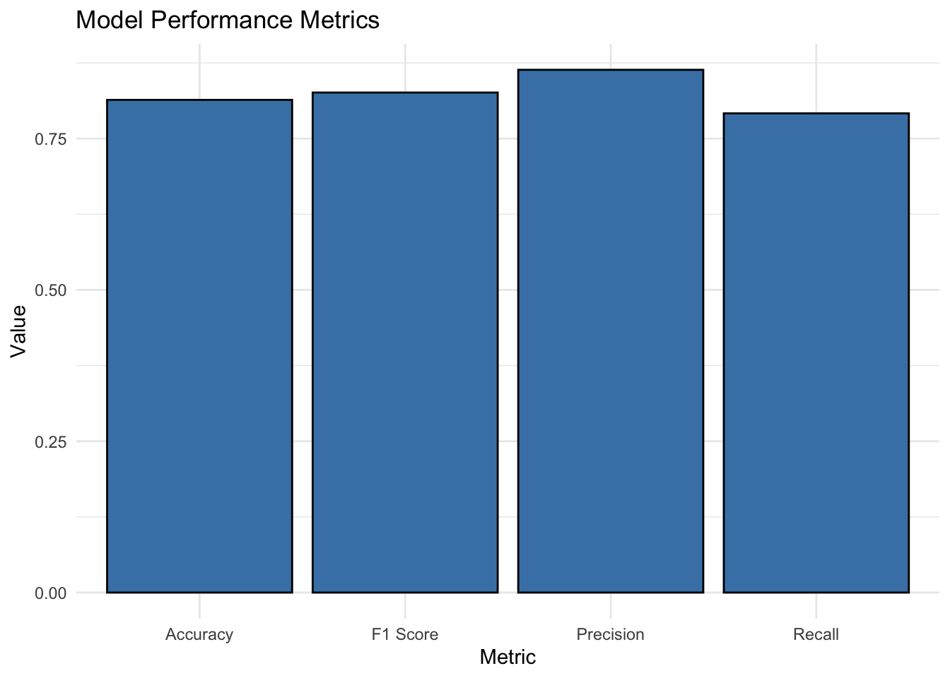

Function for computing Specificity and Sensitivity

library(purrr)

get_sens_spec <- function(threshold, score, actual, direction){

predicted <- if(direction == “greaterthan”) { score > threshold } else { score < threshold }

tp <- sum(predicted & actual) tn <- sum(!predicted & !actual) fp <- sum(predicted & !actual) fn <- sum(!predicted & actual)

specificity <- tn / (tn + fp) sensitivity <- tp / (tp + fn)

tibble(“specificity” = specificity, “sensitivity” = sensitivity) }

get_roc_data <- function(x, direction){

# x <- test # direction <- “greaterthan”

thresholds <- unique(x$score) %>% sort()

map_dfr(.x=thresholds, ~get_sens_spec(.x, x\(score, x\)srn, direction)) %>% rbind(c(specificity = 0, sensitivity = 1)) }

8.2 ROC Curve and AUC-ROC

The ROC Curve plots the true positive rate (sensitivity) against the false positive rate (1 - specificity) at various threshold settings. It provides a visual representation of the classifier’s performance across different threshold levels. The Area Under the ROC Curve (AUC-ROC) quantifies the overall performance of the model in distinguishing between the positive and negative classes. A higher AUC-ROC value indicates better discrimination performance.

library(pROC)
library(ggplot2)

# Compute predicted probabilities
predicted_probabilities <- predict(mod_regLogistic_cv, newdata = test_data, type = "prob")

# Extract probabilities for the positive class
positive_probabilities <- predicted_probabilities$"0"

# Compute ROC curve and AUC-ROC
roc_curve <- pROC::roc(test_data$target, positive_probabilities)
auc_roc <- pROC::auc(roc_curve)

# Plot ROC curve with descriptive axis titles
ggroc(roc_curve, color = "steelblue", size = 1) +
  labs(title = "Receiver Operating Characteristic (ROC) Curve",
       x = "False Positive Rate (1 - Specificity)",
       y = "True Positive Rate (Sensitivity)") +
  theme_minimal()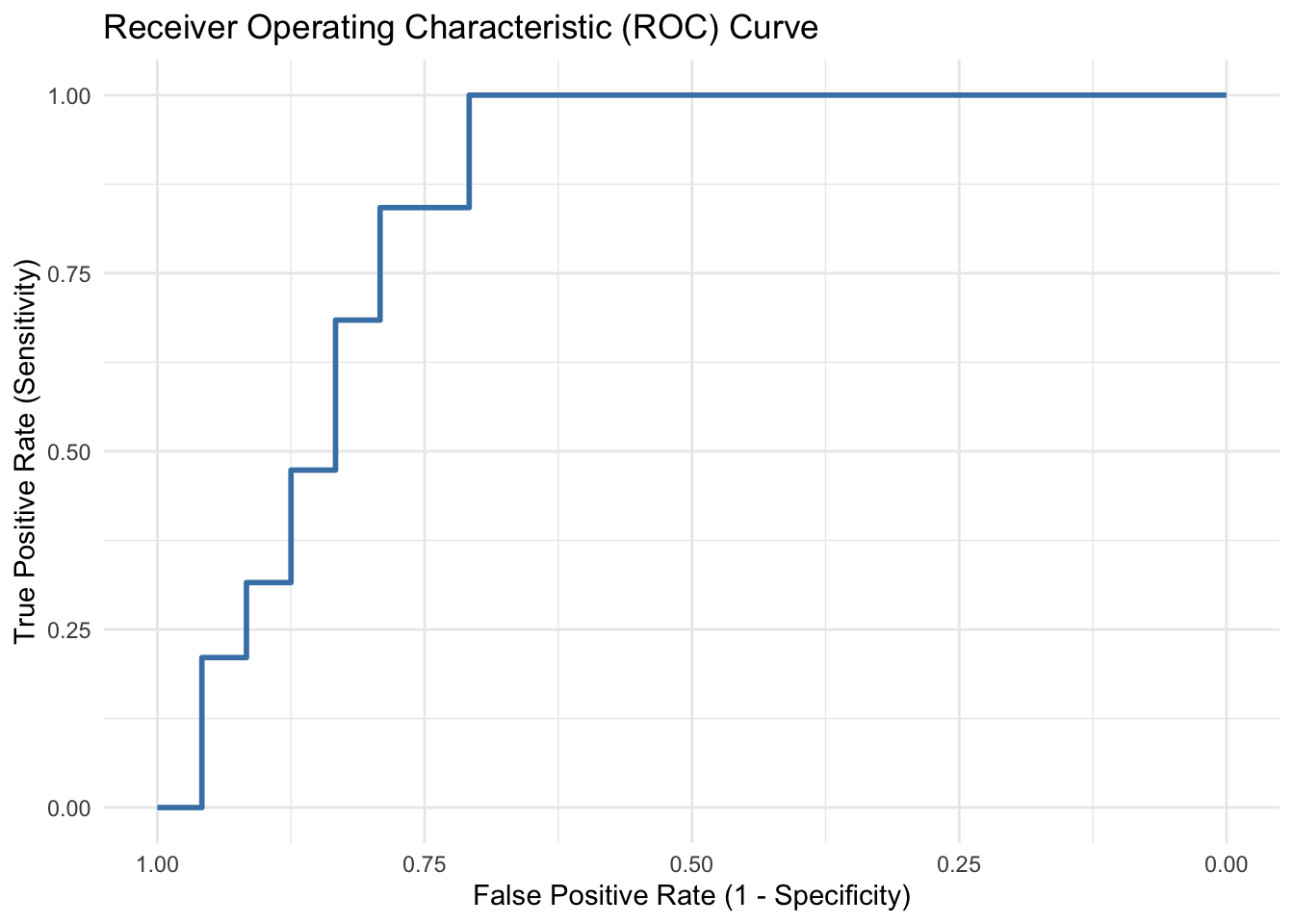

# Print AUC-ROC
cat("AUC-ROC:", auc_roc)
AUC-ROC: 0.8486842