5 Feature Engineering
Feature engineering is a crucial step in the machine learning pipeline where raw data is transformed into a format that enhances the performance of predictive models. This process involves creating new features, selecting relevant features, and transforming existing features to improve the model’s ability to capture patterns and make accurate predictions.
By performing effective feature engineering, we can improve the performance, interpretability, and robustness of machine learning models, ultimately leading to better predictions and insights from the data.
Some common techniques used in feature engineering include feature creation, selection and transformation.
5.1 Feature Creation (Simplified Example)
Feature creation involves generating new features from existing ones. This can include extracting information from text, dates, or categorical variables, or creating interaction terms between variables.
For example: In this simplified example, we demonstrate feature creation using demographic data.Here, we divide ages into three groups based on the ‘age’ column to create a new feature called ‘age_group’. We first load the necessary libraries, then create sample data containing information about age, gender, and income. We then create a new feature called age_group based on the ‘age’ column, dividing ages into three groups: “<30”, “30-40”, and “>40”. Finally, we display the DataFrame with the new feature included.
5.1.1 Sample dataframe
## ── Attaching core tidyverse packages ──────────────────────── tidyverse 2.0.0 ──
## ✔ dplyr     1.1.4     ✔ readr     2.1.5
## ✔ forcats   1.0.0     ✔ stringr   1.5.1
## ✔ ggplot2   3.5.0     ✔ tibble    3.2.1
## ✔ lubridate 1.9.3     ✔ tidyr     1.3.1
## ✔ purrr     1.0.2
## ── Conflicts ────────────────────────────────────────── tidyverse_conflicts() ──
## ✖ dplyr::filter() masks stats::filter()
## ✖ dplyr::lag()    masks stats::lag()
## ℹ Use the conflicted package (<http://conflicted.r-lib.org/>) to force all conflicts to become errors
# Sample data
data <- tibble(
  age = c(25, 30, 35, 40, 45),
  gender = c('male', 'female', 'male', 'male', 'female'),
  income = c(50000, 60000, 75000, 80000, 70000)
)

# Creating a DataFrame
df <- as_tibble(data)
print(df)
## # A tibble: 5 × 3
## age gender income
## <dbl> <chr> <dbl>
## 1 25 male 50000
## 2 30 female 60000
## 3 35 male 75000
## 4 40 male 80000
## 5 45 female 700005.1.2 Creating a new feature ‘age_group’
# Feature creation example: creating a new feature 'age_group' based on age
df <- df %>%
  mutate(age_group = cut(age, breaks = c(0, 30, 40, Inf), labels = c("<30", "30-40", ">40")))

# Displaying the DataFrame with the new feature
print(df)
## # A tibble: 5 × 4
## age gender income age_group
## <dbl> <chr> <dbl> <fct>
## 1 25 male 50000 <30
## 2 30 female 60000 <30
## 3 35 male 75000 30-40
## 4 40 male 80000 30-40
## 5 45 female 70000 >40While this example demonstrates feature creation using demographic data, the same principles apply to various types of data, including metagenomics and microbiome data.
5.2 Feature Selection
Identifying the most relevant features that contribute the most to the predictive power of the model while reducing dimensionality and computational complexity.
- Objective: Perform feature selection to identify relevant microbial taxa or functional pathways associated with the binary outcome of interest, such as disease status or treatment response.
- Techniques: Utilize methods like Lasso regularization, Recursive Feature Elimination (RFE), and Boruta algorithm to automatically select important features and penalize less informative ones, enhancing model interpretability and performance.
5.3 Feature Selection Techniques
Feature selection techniques aim to identify the most relevant and informative features for modeling, reducing the dimensionality of the data while preserving predictive performance. Key techniques include:
- Variance Threshold: Eliminates features with low variance, indicating little variability and potentially less relevance to the target variable.
- Univariate Selection: Examines each feature’s relationship with the target variable independently, selecting those with the strongest statistical significance.
- Recursive Feature Elimination (RFE): Sequentially removes the least important features, based on model performance, until an optimal subset is obtained.
- Principal Component Analysis (PCA): Projects the original features into a lower-dimensional space, retaining the most critical information while reducing dimensionality.
- Feature Importance: Determines the importance of features by assessing their contribution to model performance. Techniques include Random Forest feature importance and permutation importance.
- Correlation Analysis: Identifies relationships between pairs of features, helping to detect redundant or highly correlated variables.
- Forward/Backward Selection: Iteratively adds or removes features from the model, based on their impact on performance, to arrive at the best subset.
- Least Absolute Shrinkage and Selection Operator (LASSO): Penalizes the absolute size of feature coefficients, encouraging sparse solutions and automatic feature selection.
These techniques facilitate the creation of more efficient and interpretable models by focusing on the most informative features while reducing redundancy and noise.
5.3.1 Demo using Variance threshold
- It involves calculating the variance of each feature.
- Only those features whose variance exceeds a predefined threshold are selected.
- This method is useful for filtering out features that have very low variance, indicating little variation in the data.
## Loading objects:
##   composite
##   metabo_composite
##   ml_genus_dsestate
##   ps_df
##   ml_genus_enttype
##   ml_genus_nationality
##   ml_genus_bmi
# Example dataset (replace with your own data)
data <- ml_genus_nationality
# data <- ml_genus_bmi
# data <- ml_genus_enttype
# data <- ml_genus_dsestate

# Calculate variance for each feature
variances <- apply(data[, -1], 2, var)  # Exclude the first column (nationality)

# Set the threshold for variance
threshold <- 0.0001  # Adjust as needed

# Identify features with variance above the threshold
selected_features <- names(variances[variances > threshold])

# Remove NA values from selected_features
selected_features <- selected_features[!is.na(selected_features)]

# Add the first column (nationality) to the selected features
selected_features <- c("nationality", selected_features)

# Filter dataset to include selected features
filtered_data <- data[, colnames(data) %in% selected_features]

# Display filtered dataset
head(filtered_data[1:3, 1:5])
## # A tibble: 3 × 5
## nationality Akkermansia Allistipes `Bacteroides fragilis` `Bacteroides ovatus`
## <fct> <dbl> <dbl> <dbl> <dbl>
## 1 0 0.00213 0.0397 0.0524 0.0505
## 2 1 0.00724 0.00180 0.00151 0.000637
## 3 1 0.136 0.00897 0.0729 0.005185.3.2 Demo using Correlation Analysis
- This method involves calculating the correlation between each feature and the target variable (or another feature).
- Features are then selected based on their correlation coefficients.
- A cutoff point for the correlation coefficient can be set to determine which features are considered relevant.
- Features with correlation coefficients above this cutoff are retained, while those below are discarded.
# Example dataset (replace with your own data)
data <- ml_genus_nationality

# Calculate point-biserial correlation between each feature and the categorical target variable
correlations <- sapply(data[-1], function(x) cor(x, as.numeric(data$nationality)))

# Set the threshold for correlation
threshold <- 0.3  # Adjust as needed

# Identify features with correlation above the threshold
selected_features <- names(correlations[abs(correlations) > threshold])

# Add the target variable (nationality) to the selected features
selected_features <- c("nationality", selected_features)

# Filter dataset to include selected features
filtered_data <- data[, colnames(data) %in% selected_features]

# Display filtered dataset
head(filtered_data[1:3, 1:5])
## # A tibble: 3 × 5
## nationality Allistipes `Anaerostipes caccae` `Bacteroides fragilis`
## <fct> <dbl> <dbl> <dbl>
## 1 0 0.0397 0.0288 0.0524
## 2 1 0.00180 0.00168 0.00151
## 3 1 0.00897 0.00168 0.0729
## # ℹ 1 more variable: `Bacteroides ovatus` <dbl>Note: NA values must be removed from the selected_features vector before filtering the dataset to avoid errors.
5.3.3 Demo with Wilcoxon rank sum test
The Wilcoxon rank sum test, also known as the Mann-Whitney U test, is a nonparametric test used to assess whether two independent samples have different distributions. It is particularly useful when the assumptions of the t-test are not met, such as when the data is not normally distributed or when the sample sizes are small
library(tidyverse)
library(broom)
all_genera <- composite %>%
tidyr::nest(data = -taxonomy) %>%
mutate(test = purrr::map(data, ~wilcox.test(rel_abund ~ hyper, data = .x) %>% tidy)) %>%
tidyr::unnest(test) %>%
mutate(p.adjust = p.adjust(p.value, method = "BH"))
sig_genera <- all_genera %>%
dplyr::filter(p.value < 0.001) %>%
arrange(p.adjust) %>%
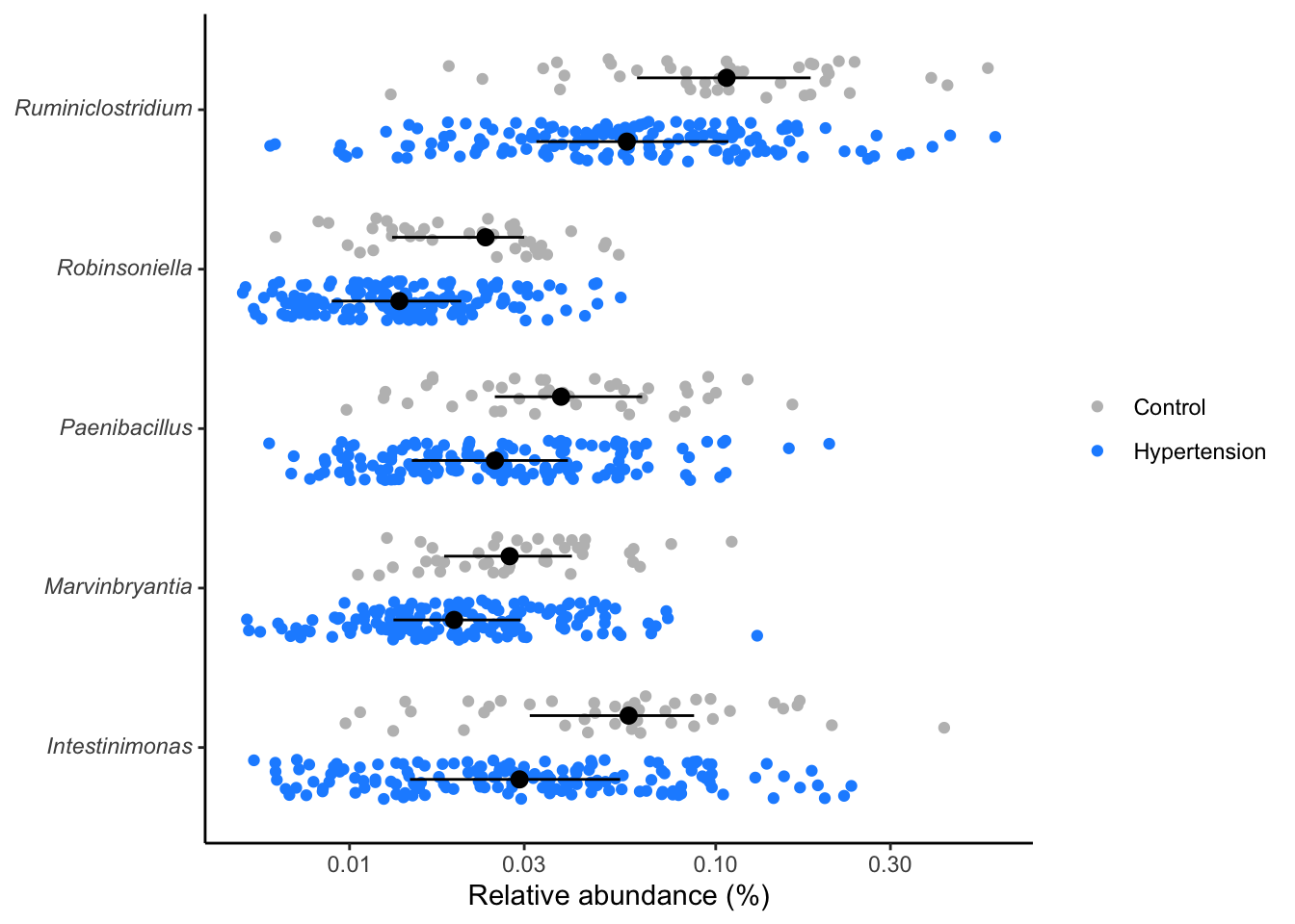
dplyr::select(taxonomy, p.value)Distribution of significant genera
- Compute the significant genera, then
- P-values or Adjusted P-values (p.adjust) can be used to measure the significance levels.
- View the distribution of the significant genera
library(tidyverse)
library(ggtext)

composite %>%
  inner_join(sig_genera, by="taxonomy") %>%
  mutate(rel_abund = 100 * (rel_abund + 1/20000),
         taxonomy = str_replace(taxonomy, "(.*)", "*\\1*"),
         taxonomy = str_replace(taxonomy, "\\*(.*)_unclassified\\*",
                                "Unclassified<br>*\\1*"),
         hyper = factor(hyper, levels = c(T, F))) %>%
  ggplot(aes(x=rel_abund, y=taxonomy, color=hyper, fill=hyper)) +
  # geom_vline(xintercept = 100/10530, size=0.5, color="gray") +
  geom_jitter(position = position_jitterdodge(dodge.width = 0.8,
                                              jitter.width = 0.5),
              shape=21) +
  stat_summary(fun.data = median_hilow, fun.args = list(conf.int=0.5),
               geom="pointrange",
               position = position_dodge(width=0.8),
               color="black", show.legend = FALSE) +
  scale_x_log10() +
  scale_color_manual(NULL,
                     breaks = c(F, T),
                     values = c("gray", "dodgerblue"),
                     labels = c("Control", "Hypertension")) +
  scale_fill_manual(NULL,
                     breaks = c(F, T),
                     values = c("gray", "dodgerblue"),
                     labels = c("Control", "Hypertension")) +
  labs(x= "Relative abundance (%)", y=NULL) +
  theme_classic() +
  theme(
    axis.text.y = element_markdown()
  )
ggsave("figures/significant_genera.tiff", width=6, height=4)
library(tidyverse)

# Compute the significant pathways using `wilcox.test`.
all_metabopwy <- metabo_composite %>%
  tidyr::nest(data = -metabopwy) %>%
  mutate(test = purrr::map(.x=data, ~wilcox.test(rel_abund~hyper, data=.x) %>% tidy)) %>%
  tidyr::unnest(test) %>%
  mutate(p.adjust = p.adjust(p.value, method="BH"))

sig_metabopwy <- all_metabopwy %>%
  dplyr::filter(p.value < 0.3) %>% # Typically, the best significant p-value is set at 0.05
  dplyr::select(metabopwy, p.value)
Distribution of significant metabolic pathways
- Compute the significant pathways, then
- P-values or Adjusted P-values (p.adjust) can be used to measure the significance levels.
- View the distribution of the significant pathways.
metabo_composite %>%
  inner_join(sig_metabopwy, by="metabopwy") %>%
  mutate(rel_abund = 100 * (rel_abund + 1/20000),
         metabopwy = str_replace(metabopwy, "(.*)", "*\\1*"),
         metabopwy = str_replace(metabopwy, "\\*(.*)_unclassified\\*",
                                "Unclassified<br>*\\1*"),
         hyper = factor(hyper, levels = c(T, F))) %>%
  ggplot(aes(x=rel_abund, y=metabopwy, color=hyper, fill=hyper)) +
  geom_jitter(position = position_jitterdodge(dodge.width = 0.8,
                                              jitter.width = 0.5),
              shape=21) +
  stat_summary(fun.data = median_hilow, fun.args = list(conf.int=0.5),
               geom="pointrange",
               position = position_dodge(width=0.8),
               color="black", show.legend = FALSE) +
  scale_x_log10() +
  scale_color_manual(NULL,
                     breaks = c(F, T),
                     values = c("gray", "dodgerblue"),
                     labels = c("Control", "Hypertension")) +
  scale_fill_manual(NULL,
                     breaks = c(F, T),
                     values = c("gray", "dodgerblue"),
                     labels = c("Control", "Hypertension")) +
  labs(x= "Relative abundance (%)", y=NULL) +
  theme_classic() +
  theme(
    axis.text.y = element_markdown()
  )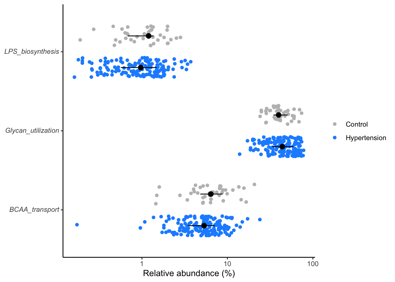
ggsave("figures/significant_genera.tiff", width=6, height=4)Here we filter the metabolic pathways at a lesser stringent
p.values(p < 0.25) for demo purposes.
5.4 Feature Transformation:
- Applying transformations to features to make the data more suitable for modeling.
- Scaling numeric features ensures that all features contribute equally to the analysis by bringing them to a similar scale.
- Encoding categorical variables converts categorical data into a numerical format, allowing algorithms to work with categorical data.
- Handling missing values involves strategies such as imputation or removal of missing data to ensure completeness of the dataset.
library(tidyverse)

# Load the dataset
data <- ml_genus_nationality %>%
  dplyr::rename(target = nationality)

# Check for missing values
missing_values <- colSums(is.na(data))

# Impute missing values with zeros
data_imputed <- replace(data, is.na(data), 0)

# Display the first few rows of the imputed dataset
head(data_imputed[1:3, 1:5])
# A tibble: 3 × 5
  target Actinobacteria Akkermansia `Alcaligenes faecalis` Allistipes
  <fct>           <dbl>       <dbl>                  <dbl>      <dbl>
1 0            0.00121      0.00213               0.000118    0.0397
2 1            0.000533     0.00724               0.000406    0.00180
3 1            0.00123      0.136                 0.000420    0.00897

save(data_imputed, file = "data/data_imputed.rda")